这是笔者在github上开源的(又)一个小项目,已经有9个小星星啦,链接:Retinal Vessel Segmentation,在此分享给大家,当然,也还有可以优化的地方,欢迎讨论!
图像分割
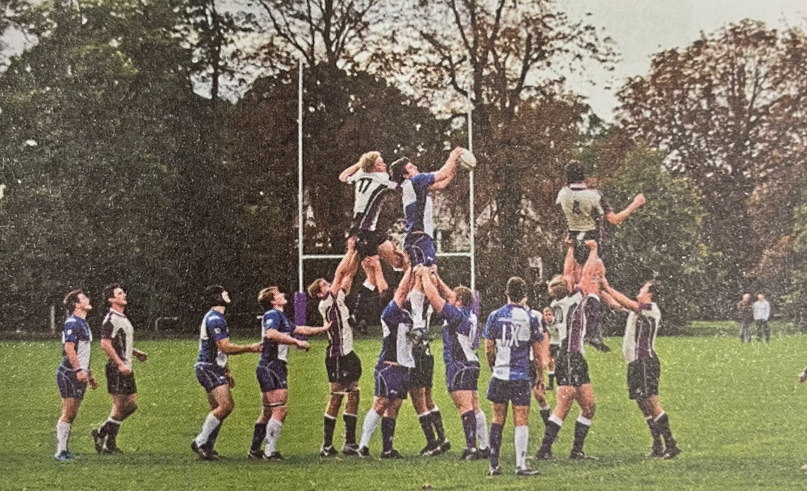
图像分割(Image Segmentation)是计算机视觉领域的经典问题之一,是将数字图像细分为多个图像子区域(像素的集合)的过程。
-
图像分割用于预测图像中每个像素点所属的类别或实体。基于深度学习的图像分割主要分为三类
-
语义分割
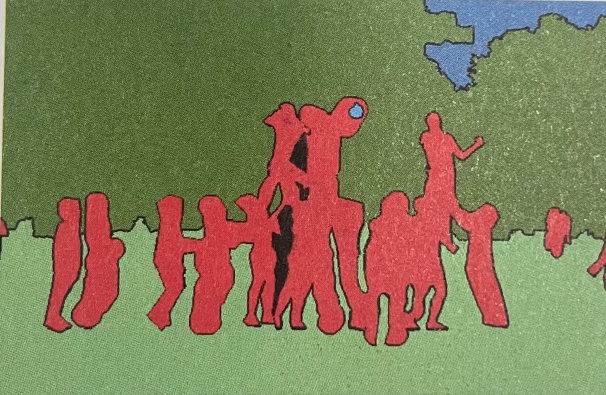
语义分割(Semantic Segmentation)就是按照“语义”为图像上的每个像素点打一个标签,是像素级别的分类任务。
-
实例分割
实例分割(Instance Segmentation)就是在像素级别分类的基础上,进一步区分具体类别上不同的实例。
-
全景分割
全景分割(Panoramic Segmentation)是对图中的所有对象(包括背景)都要进行检测和分割。
-
语义分割
语义分割是一项计算机视觉任务,旨在对输入图像中的每个像素进行分类,从而生成一张语义标注图。具体来说,对于一幅 RGB 彩色图像(尺寸为 H × W × C=3)或 灰度图像(H × W × C=1),语义分割模型的输出是一个尺寸为 H × W × 1 的分割图谱,其中每个像素被分配一个类别标签。
1. 分割标注的基本要求
在实际应用中,分割标注的 分辨率 需要与原始输入图像一致,以确保精确像素级分类。
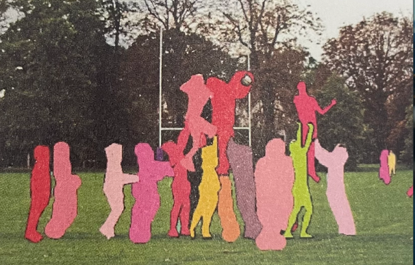
2. 类别定义
在目标分割任务中,图像中的物体通常被划分为多个类别,例如:
- Person(人)
- Purse(包)
- Plant/Grass(植物/草地)
- Building/Structure(建筑/结构)
- Sidewalk(人行道)
每个类别的像素点需要被正确标注,以形成精确的分割结果。
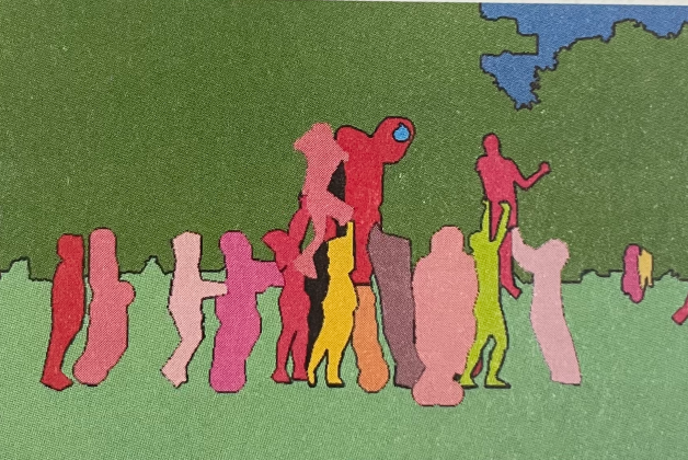
3. One-hot 编码与掩码(Mask)
语义分割的标注采用 One-hot 编码 方式,每个类别对应一个单独的通道。例如,假设输入图像有 H × W 像素,输出的标签数据会有 H × W × N 维度(其中 N 是类别数)。在 One-hot 编码中:
- 每个通道仅包含 0 或 1。
- 对于 Person(人) 这一通道,值为 1 的像素表示该位置属于 “Person”,其余像素均为 0。
- 不会 存在一个像素点同时属于多个类别,即同一像素点不会在多个通道中同时为 1。
4. 类别预测与 Mask 生成
在推理过程中,可以使用 Argmax 函数对每个像素点的通道值进行计算,找到概率最高的类别索引,从而确定该像素的最终分类。
此外,某个类别的通道可以与原始图像叠加,形成 Mask(掩码),直观地表示该类别在图像中的分布。例如,在人物检测任务中,Person 通道的 mask 可以覆盖原始图像中所有属于 “Person” 类别的像素区域。
全卷积神经网络
全卷积神经网络(Fully Convolutional Netwvork, FCN)把普通卷积神经网络后面几个全连接都换成卷积层,最终得到一个二维的特征映射图,并使用Softmax 层获得每个像素点的分类信息,从而解决分割问题。
在卷积神经网络中,经过多次卷积和池化以后,得到的图像越来越小,分辨率越来越低,直到获得高维特征图。图像分割在得到高维特征图之后需要进行上采样,把图像放大到原图像的大小。
反卷积
反卷积(Deconvolution)的参数和卷积神经网络的参数一样,是在训练全卷积神经网络的过程中通过BP 算法得到的。
反卷积的参数利用卷积过程Filter的转置作为计算卷积前的特征图。
U-Net模型
U-Net 是一种 全卷积神经网络(Fully Convolutional Network, FCN),广泛应用于医学影像处理,尤其是在 脑血管分割 等任务中表现出色。其核心特点在于 U 形结构 和 跳层连接(Skip Connections),能够有效提高分割精度。
1. U-Net 结构解析
U-Net 由 编码(Encoder) 和 解码(Decoder) 两部分组成:
- 左侧(编码路径 / 下采样)
- 由 卷积层 + 池化层 组成,类似于传统 CNN 结构。
- 逐步提取图像特征,同时减少空间分辨率,捕捉高层语义信息。
- 右侧(解码路径 / 上采样)
- 通过 反卷积(转置卷积)或插值上采样 逐步恢复分辨率。
- 每次上采样后,与编码路径的对应层进行 跳层连接(Skip Connection),保留空间细节,提高分割精度。
- 跳层连接(Skip Connections)
- 直接连接编码部分和解码部分的相应层,以弥补上采样过程中信息的丢失。
- 例如,在标准 U-Net 结构中,通常包含 4 次跳层连接,确保高分辨率特征能够被有效传递。
2. U-Net 在图像分割中的应用
在语义分割任务中,U-Net 主要用于生成 掩码(Mask),即将目标区域从背景中分离出来。例如,在医学影像分割中,可以用 U-Net 精确地提取肿瘤、血管或其他病灶区域。
为了存储和处理分割结果,U-Net 采用 RLE(Run-Length Encoding)压缩方法。
- RLE(长度编码压缩)原理
- 对连续相同的像素值进行编码,仅存储其 值 和 重复次数。
- 例如,字符串
aaabccccccddeee经过 RLE 编码后变为3a1b6c2d3e。 - 适用于大面积 相同类别的区域,能有效减少存储需求。
3. U-Net 之外的其他分割网络
除了 U-Net,图像分割领域还出现了多种基于深度学习的模型,包括:
- SegNet:采用基于 池化索引(Pooling Indexes) 进行上采样,提高计算效率。
- DeconvNet:基于 反卷积(Deconvolution) 进行逐步恢复分辨率,适用于高精度分割任务。
U-Net 及其变体(如 ResUNet、Attention U-Net)在医学影像、卫星遥感、自动驾驶等多个领域均被广泛使用,并且仍然是 像素级分割任务的经典选择。
代码
使用 U-Net 模型训练眼度血管数据集(DRIVE),然后使用训练好的模型进行眼底血管图像分割,完整步骤如下:
1. 生成数据集(dataset.py)
import os
import numpy as np
import cv2
from glob import glob
from tqdm import tqdm
import imageio
from albumentations import HorizontalFlip, VerticalFlip, Rotate

""" Create a directory """
def create_dir(path):
    if not os.path.exists(path):
        os.makedirs(path)

def load_data(path):
    train_x = sorted(glob(os.path.join(path, "training", "images", "*.tif")))
    train_y = sorted(glob(os.path.join(path, "training", "1st_manual", "*.gif")))

    test_x = sorted(glob(os.path.join(path, "test", "images", "*.tif")))
    test_y = sorted(glob(os.path.join(path, "test", "1st_manual", "*.gif")))

    return (train_x, train_y), (test_x, test_y)

def augment_data(images, masks, save_path, augment=True):
    size = (512, 512)

    for idx, (x, y) in tqdm(enumerate(zip(images, masks)), total=len(images)):
        """ Extracting the name """
        name = os.path.splitext(os.path.basename(x))[0]

        """ Reading image and mask """
        x = cv2.imread(x, cv2.IMREAD_COLOR)
        y = imageio.mimread(y)[0]

        if augment:
            aug = HorizontalFlip(p=1.0)
            augmented = aug(image=x, mask=y)
            x1 = augmented["image"]
            y1 = augmented["mask"]

            aug = VerticalFlip(p=1.0)
            augmented = aug(image=x, mask=y)
            x2 = augmented["image"]
            y2 = augmented["mask"]

            aug = Rotate(limit=45, p=1.0)
            augmented = aug(image=x, mask=y)
            x3 = augmented["image"]
            y3 = augmented["mask"]

            X = [x, x1, x2, x3]
            Y = [y, y1, y2, y3]

        else:
            X = [x]
            Y = [y]

        index = 0
        for i, m in zip(X, Y):
            i = cv2.resize(i, size)
            m = cv2.resize(m, size)

            tmp_image_name = f"{name}_{index}.png"
            tmp_mask_name = f"{name}_{index}.png"

            image_path = os.path.join(save_path, "image", tmp_image_name)
            mask_path = os.path.join(save_path, "mask", tmp_mask_name)

            cv2.imwrite(image_path, i)
            cv2.imwrite(mask_path, m)

            index += 1

if __name__ == "__main__":
    """ Seeding """
    np.random.seed(42)

    """ Load the data """
    data_path = "DRIVE"
    (train_x, train_y), (test_x, test_y) = load_data(data_path)

    print(f"Train: {len(train_x)} - {len(train_y)}")
    print(f"Test: {len(test_x)} - {len(test_y)}")

    """ Create directories to save the augmented data """
    create_dir(os.path.join("data", "train", "image"))
    create_dir(os.path.join("data", "train", "mask"))
    create_dir(os.path.join("data", "test", "image"))
    create_dir(os.path.join("data", "test", "mask"))

    """ Data augmentation """
    augment_data(train_x, train_y, os.path.join("data", "train"), augment=True)
    augment_data(test_x, test_y, os.path.join("data", "test"), augment=False)
这段代码主要用于 加载、预处理和增强医学图像数据(如 DRIVE 数据集中的视网膜血管分割任务)。其核心流程如下:
- 创建目录 (
create_dir):确保存储增强后数据的目录存在。 - 加载数据 (
load_data):读取训练集和测试集的图像(.tif)及其对应的掩码(.gif)。 - 数据增强 (
augment_data):- 读取图像和掩码,并进行 水平翻转、垂直翻转、随机旋转(45°)。
- 生成多个增强版本的图像及掩码,统一调整大小至
(512, 512)。 - 以
name_index.png形式保存到指定路径(image/和mask/)。
- 主函数 (
__main__):- 设定随机种子,确保可复现性。
- 读取数据并打印数据集大小。
- 创建存储增强数据的文件夹。
- 进行数据增强(训练集增强 3 倍,测试集不增强)。
2. 数据预处理(preprocess.py)
import os
import numpy as np
import cv2
import torch
from torch.utils.data import Dataset

class DriveDataset(Dataset):
    def __init__(self, images_path, masks_path):

        self.images_path = images_path
        self.masks_path = masks_path
        self.n_samples = len(images_path)

    def __getitem__(self, index):
        """ Reading image """
        image = cv2.imread(self.images_path[index], cv2.IMREAD_COLOR)
        image = image/255.0 ## (512, 512, 3)
        image = np.transpose(image, (2, 0, 1))  ## (3, 512, 512)
        image = image.astype(np.float32)
        image = torch.from_numpy(image)

        """ Reading mask """
        mask = cv2.imread(self.masks_path[index], cv2.IMREAD_GRAYSCALE)
        mask = mask/255.0   ## (512, 512)
        mask = np.expand_dims(mask, axis=0) ## (1, 512, 512)
        mask = mask.astype(np.float32)
        mask = torch.from_numpy(mask)

        return image, mask

    def __len__(self):
        return self.n_samples
这段代码定义了一个 PyTorch 自定义数据集类 (DriveDataset),用于加载 医学图像分割数据集,其核心功能如下:
- 初始化 (
__init__)- 接收 图像路径列表 和 掩码路径列表,并计算数据样本数量。
- 获取单个样本 (
__getitem__)- 读取图像(
cv2.imread以彩色格式加载),归一化至[0,1],并转换为 (C, H, W) 格式的 PyTorch 张量 (torch.Tensor)。 - 读取掩码(以灰度模式加载),归一化至
[0,1],并添加通道维度 (1, H, W) 以适配网络输入格式。
- 读取图像(
- 获取数据集大小 (
__len__)- 返回数据集的样本总数。
3. 构建U-Net模型(model.py和loss.py)
import torch
import torch.nn as nn

class conv_block(nn.Module):
    def __init__(self, in_c, out_c):
        super().__init__()

        self.conv1 = nn.Conv2d(in_c, out_c, kernel_size=3, padding=1)
        self.bn1 = nn.BatchNorm2d(out_c)

        self.conv2 = nn.Conv2d(out_c, out_c, kernel_size=3, padding=1)
        self.bn2 = nn.BatchNorm2d(out_c)

        self.relu = nn.ReLU()

    def forward(self, inputs):
        x = self.conv1(inputs)
        x = self.bn1(x)
        x = self.relu(x)

        x = self.conv2(x)
        x = self.bn2(x)
        x = self.relu(x)

        return x

class encoder_block(nn.Module):
    def __init__(self, in_c, out_c):
        super().__init__()

        self.conv = conv_block(in_c, out_c)
        self.pool = nn.MaxPool2d((2, 2))

    def forward(self, inputs):
        x = self.conv(inputs)
        p = self.pool(x)

        return x, p

class decoder_block(nn.Module):
    def __init__(self, in_c, out_c):
        super().__init__()

        self.up = nn.ConvTranspose2d(in_c, out_c, kernel_size=2, stride=2, padding=0)
        self.conv = conv_block(out_c+out_c, out_c)

    def forward(self, inputs, skip):
        x = self.up(inputs)
        x = torch.cat([x, skip], axis=1)
        x = self.conv(x)
        return x

class build_unet(nn.Module):
    def __init__(self):
        super().__init__()

        """ Encoder """
        self.e1 = encoder_block(3, 64)
        self.e2 = encoder_block(64, 128)
        self.e3 = encoder_block(128, 256)
        self.e4 = encoder_block(256, 512)

        """ Bottleneck """
        self.b = conv_block(512, 1024)

        """ Decoder """
        self.d1 = decoder_block(1024, 512)
        self.d2 = decoder_block(512, 256)
        self.d3 = decoder_block(256, 128)
        self.d4 = decoder_block(128, 64)

        """ Classifier """
        self.outputs = nn.Conv2d(64, 1, kernel_size=1, padding=0)

    def forward(self, inputs):
        """ Encoder """
        s1, p1 = self.e1(inputs)
        s2, p2 = self.e2(p1)
        s3, p3 = self.e3(p2)
        s4, p4 = self.e4(p3)

        """ Bottleneck """
        b = self.b(p4)

        """ Decoder """
        d1 = self.d1(b, s4)
        d2 = self.d2(d1, s3)
        d3 = self.d3(d2, s2)
        d4 = self.d4(d3, s1)

        outputs = self.outputs(d4)

        return outputs

if __name__ == "__main__":
    x = torch.randn((2, 3, 512, 512))
    f = build_unet()
    y = f(x)
print(y.shape)
这段代码实现了 U-Net 语义分割模型,核心结构如下:
- 基础卷积模块 (
conv_block):- 由两个 3×3 卷积 + 批归一化(BN)+ ReLU 组成,提取特征。
- 编码器 (
encoder_block):- 使用
conv_block进行特征提取后,采用 2×2 最大池化(MaxPool2d) 降低特征图尺寸。
- 使用
- 解码器 (
decoder_block):- 采用 转置卷积(ConvTranspose2d) 进行上采样。
- 跳跃连接(Skip Connection)拼接编码层特征后,再通过
conv_block处理。
- U-Net 结构 (
build_unet):- 编码阶段:4 层
encoder_block,特征通道依次增加 (3→64→128→256→512)。 - 瓶颈层:
conv_block处理 512 → 1024。 - 解码阶段:4 层
decoder_block,特征通道依次减少 (1024→512→256→128→64)。 - 输出层:
1×1卷积降维至 单通道掩码输出(1表示二分类任务)。
- 编码阶段:4 层
- 测试:
- 随机输入 (2, 3, 512, 512) 大小的张量,验证模型前向传播,输出形状为 (2, 1, 512, 512)。
import torch
import torch.nn as nn
import torch.nn.functional as F

class DiceLoss(nn.Module):
    def __init__(self, weight=None, size_average=True):
        super(DiceLoss, self).__init__()

    def forward(self, inputs, targets, smooth=1):

        #comment out if your model contains a sigmoid or equivalent activation layer
        inputs = torch.sigmoid(inputs)

        #flatten label and prediction tensors
        inputs = inputs.view(-1)
        targets = targets.view(-1)

        intersection = (inputs * targets).sum()
        dice = (2.*intersection + smooth)/(inputs.sum() + targets.sum() + smooth)

        return 1 - dice

class DiceBCELoss(nn.Module):
    def __init__(self, weight=None, size_average=True):
        super(DiceBCELoss, self).__init__()

    def forward(self, inputs, targets, smooth=1):

        #comment out if your model contains a sigmoid or equivalent activation layer
        inputs = torch.sigmoid(inputs)

        #flatten label and prediction tensors
        inputs = inputs.view(-1)
        targets = targets.view(-1)

        intersection = (inputs * targets).sum()
        dice_loss = 1 - (2.*intersection + smooth)/(inputs.sum() + targets.sum() + smooth)
        BCE = F.binary_cross_entropy(inputs, targets, reduction='mean')
        Dice_BCE = BCE + dice_loss

        return Dice_BCE
这段代码定义了 DiceLoss 和 DiceBCELoss 损失函数,适用于 二分类语义分割任务,核心功能如下:
DiceLoss(Dice 系数损失):- 计算 Dice 系数,用于衡量预测结果与目标的相似度。
- 先对输入进行 Sigmoid 激活(确保概率值)。
-
将输入和目标展平成一维,计算交集并归一化:
\[\text{Dice} = \frac{2 \times |A \cap B| + \text{smooth}}{|A| + |B| + \text{smooth}}\] - 目标是 最大化 Dice 系数,因此返回
1 - Dice作为损失值(Dice 越高损失越小)。
DiceBCELoss(Dice + BCE 组合损失):-
结合 二元交叉熵(BCE) 和 DiceLoss,兼顾像素级概率误差和形状匹配误差:
\[\text{Loss} = \text{BCE} + (1 - \text{Dice})\] -
BCE 关注单个像素的预测概率,而 Dice 关注全局匹配程度,二者结合提高分割稳定性。
-
4. 模型训练(train.py和utils.py)
import os
import time
from glob import glob
import torch
from torch.utils.data import DataLoader
import torch.nn as nn
from preprocess import DriveDataset
from model import build_unet
from loss import DiceLoss, DiceBCELoss
from utils import seeding, create_dir, epoch_time
def train(model, loader, optimizer, loss_fn, device):
epoch_loss = 0.0
model.train()
for x, y in loader:
x = x.to(device, dtype=torch.float32)
y = y.to(device, dtype=torch.float32)
optimizer.zero_grad()
y_pred = model(x)
loss = loss_fn(y_pred, y)
loss.backward()
optimizer.step()
epoch_loss += loss.item()
epoch_loss = epoch_loss/len(loader)
return epoch_loss
def evaluate(model, loader, loss_fn, device):
epoch_loss = 0.0
model.eval()
with torch.no_grad():
for x, y in loader:
x = x.to(device, dtype=torch.float32)
y = y.to(device, dtype=torch.float32)
y_pred = model(x)
loss = loss_fn(y_pred, y)
epoch_loss += loss.item()
epoch_loss = epoch_loss/len(loader)
return epoch_loss
if __name__ == "__main__":
""" Seeding """
seeding(42)
""" Directories """
create_dir("files")
""" Load dataset """
train_x = sorted(glob("data/train/image/*"))
train_y = sorted(glob("data/train/mask/*"))
valid_x = sorted(glob("data/test/image/*"))
valid_y = sorted(glob("data/test/mask/*"))
data_str = f"Dataset Size:\nTrain: {len(train_x)} - Valid: {len(valid_x)}\n"
print(data_str)
""" Hyperparameters """
H = 512
W = 512
size = (H, W)
batch_size = 2
num_epochs = 50
lr = 1e-4
checkpoint_path = "files/checkpoint.pth"
""" Dataset and loader """
train_dataset = DriveDataset(train_x, train_y)
valid_dataset = DriveDataset(valid_x, valid_y)
train_loader = DataLoader(
dataset=train_dataset,
batch_size=batch_size,
shuffle=True,
num_workers=2
)
valid_loader = DataLoader(
dataset=valid_dataset,
batch_size=batch_size,
shuffle=False,
num_workers=2
)
device = torch.device('cuda')
model = build_unet()
model = model.to(device)
optimizer = torch.optim.Adam(model.parameters(), lr=lr)
scheduler = torch.optim.lr_scheduler.ReduceLROnPlateau(optimizer, 'min', patience=5, verbose=True)
loss_fn = DiceBCELoss()
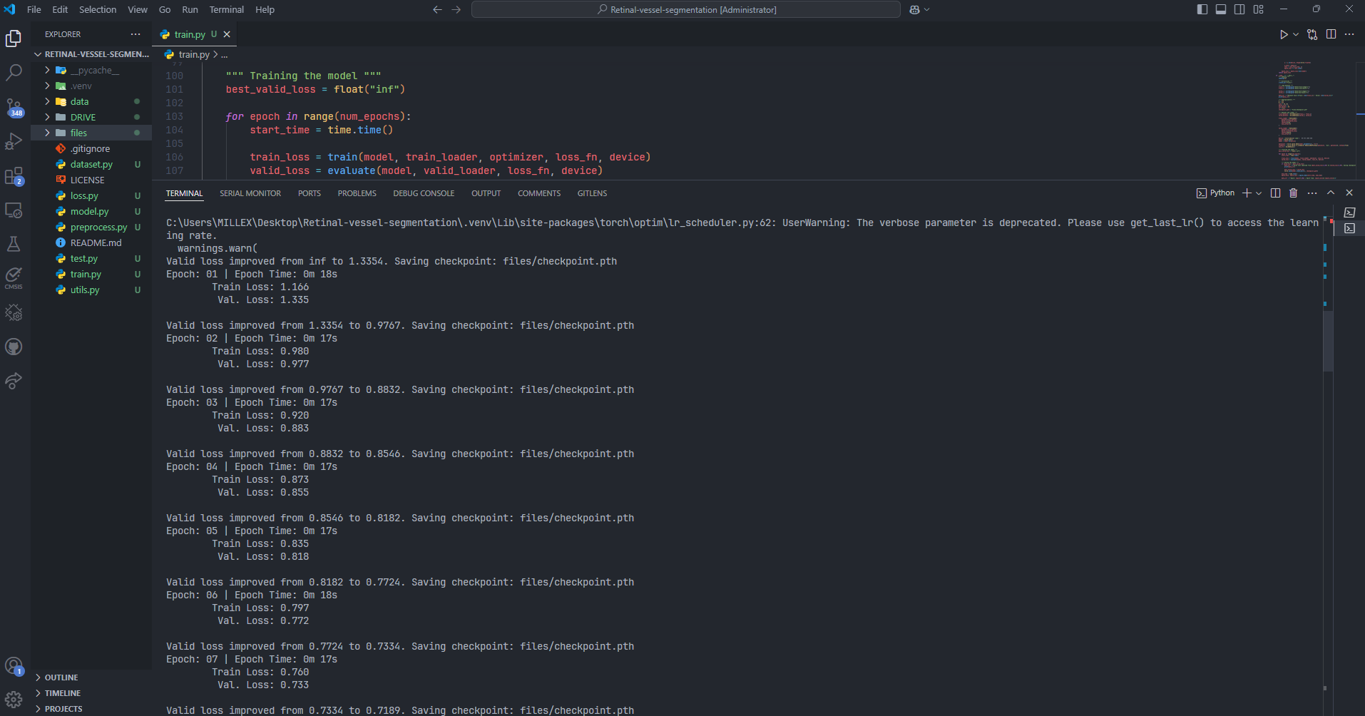
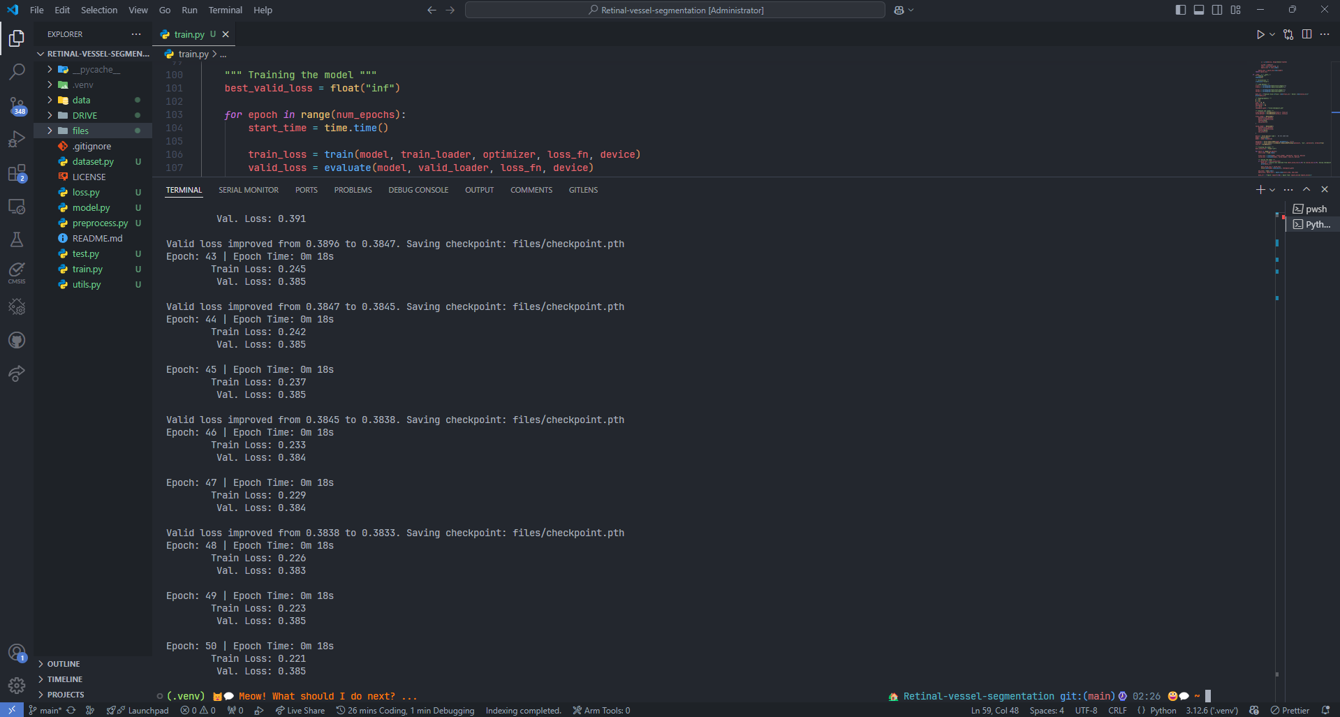
""" Training the model """
best_valid_loss = float("inf")
for epoch in range(num_epochs):
start_time = time.time()
train_loss = train(model, train_loader, optimizer, loss_fn, device)
valid_loss = evaluate(model, valid_loader, loss_fn, device)
""" Saving the model """
if valid_loss < best_valid_loss:
data_str = f"Valid loss improved from {best_valid_loss:2.4f} to {valid_loss:2.4f}. Saving checkpoint: {checkpoint_path}"
print(data_str)
best_valid_loss = valid_loss
torch.save(model.state_dict(), checkpoint_path)
end_time = time.time()
epoch_mins, epoch_secs = epoch_time(start_time, end_time)
data_str = f'Epoch: {epoch+1:02} | Epoch Time: {epoch_mins}m {epoch_secs}s\n'
data_str += f'\tTrain Loss: {train_loss:.3f}\n'
data_str += f'\t Val. Loss: {valid_loss:.3f}\n'
print(data_str)
- 训练与评估
train():执行 前向传播、计算损失、反向传播、参数更新,累积整个 epoch 的平均损失。evaluate():在torch.no_grad()下执行 前向传播,计算验证集损失。
- 训练主流程
- 设置随机种子 (
seeding(42)),保证可复现性。 - 创建保存模型的目录 (
create_dir("files"))。 - 加载数据集,包括 训练集和验证集 的图像与掩码文件路径。
- 定义超参数(
batch_size=2,num_epochs=50,lr=1e-4)。 - 构建数据加载器 (
DataLoader),以batch_size=2进行批量加载。 - 定义模型:
- U-Net (
build_unet()),加载到 GPU (cuda) 训练。 - Adam 优化器(学习率
1e-4)。 - ReduceLROnPlateau 学习率调度器(验证集损失不下降
5轮后降低学习率)。 - DiceBCELoss 作为损失函数(结合 Dice Loss 和 BCE Loss)。
- U-Net (
- 设置随机种子 (
- 训练循环
- 遍历
num_epochs轮:- 计算 训练损失 和 验证损失。
- 保存最佳模型权重(如果验证损失下降)。
- 记录 每轮训练时间 (
epoch_time()计算时间)。 - 打印 训练和验证损失。
- 遍历
- 检查点机制
- 自动保存最优模型 (
torch.save(model.state_dict(), checkpoint_path)),确保最终保留最低验证损失的模型。
- 自动保存最优模型 (
import os
import time
import random
import numpy as np
import cv2
import torch

""" Seeding the randomness. """
def seeding(seed):
    random.seed(seed)
    os.environ["PYTHONHASHSEED"] = str(seed)
    np.random.seed(seed)
    torch.manual_seed(seed)
    torch.cuda.manual_seed(seed)
    torch.backends.cudnn.deterministic = True

""" Create a directory. """
def create_dir(path):
    if not os.path.exists(path):
        os.makedirs(path)

""" Calculate the time taken """
def epoch_time(start_time, end_time):
    elapsed_time = end_time - start_time
    elapsed_mins = int(elapsed_time / 60)
    elapsed_secs = int(elapsed_time - (elapsed_mins * 60))
return elapsed_mins, elapsed_secs
这段代码提供了 训练过程中的辅助函数,主要功能如下:
- 随机种子设定 (
seeding())- 确保
random、numpy、torch生成的随机数一致,保证实验可复现性。 - 设置 CUDA 随机种子,并固定
cuDNN的计算方式以确保确定性。
- 确保
- 创建目录 (
create_dir())- 检查 指定路径是否存在,若不存在则创建该目录,方便存储模型或数据。
- 计算训练时间 (
epoch_time())- 计算 epoch 运行时间(分钟 & 秒),便于训练过程中的时间管理。
5. 模型评估(test.py)
import os
import time
from operator import add
import numpy as np
from glob import glob
import cv2
from tqdm import tqdm
import torch
from sklearn.metrics import accuracy_score, f1_score, jaccard_score, precision_score, recall_score

from model import build_unet
from utils import create_dir, seeding

def calculate_metrics(y_true, y_pred):
    """ Calculate evaluation metrics """
    y_true = y_true.cpu().numpy().astype(np.uint8).reshape(-1)
    y_pred = (y_pred.cpu().numpy() > 0.5).astype(np.uint8).reshape(-1)

    score_jaccard = jaccard_score(y_true, y_pred)
    score_f1 = f1_score(y_true, y_pred)
    score_recall = recall_score(y_true, y_pred)
    score_precision = precision_score(y_true, y_pred)
    score_acc = accuracy_score(y_true, y_pred)

    return [score_jaccard, score_f1, score_recall, score_precision, score_acc]

def mask_parse(mask):
    """ Convert grayscale mask to RGB """
    mask = np.expand_dims(mask, axis=-1)  # (H, W, 1)
    mask = np.concatenate([mask, mask, mask], axis=-1)  # (H, W, 3)
    return mask

if __name__ == "__main__":
    """ Seeding """
    seeding(42)

    """ Folders """
    results_dir = os.path.join("results")
    create_dir(results_dir)

    """ Load dataset """
    test_x = sorted(glob(os.path.join("data", "test", "image", "*")))
    test_y = sorted(glob(os.path.join("data", "test", "mask", "*")))

    assert len(test_x) > 0, "No test images found. Check 'data/test/image/' directory."
    assert len(test_y) > 0, "No test masks found. Check 'data/test/mask/' directory."

    """ Hyperparameters """
    H, W = 512, 512
    size = (W, H)
    checkpoint_path = os.path.join("files", "checkpoint.pth")
    assert os.path.exists(checkpoint_path), f"Checkpoint not found at {checkpoint_path}"

    """ Load the checkpoint """
    device = torch.device("cuda" if torch.cuda.is_available() else "cpu")

    model = build_unet()
    model = model.to(device)
    model.load_state_dict(torch.load(checkpoint_path, map_location=device))
    model.eval()

    metrics_score = [0.0, 0.0, 0.0, 0.0, 0.0]
    time_taken = []

    for i, (x, y) in tqdm(enumerate(zip(test_x, test_y)), total=len(test_x)):
        try:
            """ Extract the name """
            name = os.path.splitext(os.path.basename(x))[0]

            """ Reading image """
            image = cv2.imread(x, cv2.IMREAD_COLOR)  # (H, W, 3)
            if image is None:
                print(f"Failed to read image: {x}")
                continue
            image = cv2.resize(image, size)
            x_input = np.transpose(image, (2, 0, 1))  # (3, H, W)
            x_input = x_input / 255.0
            x_input = np.expand_dims(x_input, axis=0).astype(np.float32)  # (1, 3, H, W)
            x_input = torch.from_numpy(x_input).to(device)

            """ Reading mask """
            mask = cv2.imread(y, cv2.IMREAD_GRAYSCALE)  # (H, W)
            if mask is None:
                print(f"Failed to read mask: {y}")
                continue
            mask = cv2.resize(mask, size)
            mask_np = mask / 255.0  # Normalize mask for visualization

            y_target = np.expand_dims(mask, axis=0)  # (1, H, W)
            y_target = np.expand_dims(y_target, axis=0) / 255.0  # (1, 1, H, W)
            y_target = torch.from_numpy(y_target.astype(np.float32)).to(device)

            with torch.no_grad():
                """ Prediction and calculating FPS """
                start_time = time.time()
                pred_y = model(x_input)
                pred_y = torch.sigmoid(pred_y)
                total_time = time.time() - start_time
                time_taken.append(total_time)

                """ Calculate metrics """
                score = calculate_metrics(y_target, pred_y)
                metrics_score = list(map(add, metrics_score, score))

                """ Post-process prediction """
                pred_y = pred_y[0].cpu().numpy().squeeze()  # (H, W)
                pred_y = (pred_y > 0.5).astype(np.uint8)  # Binary mask

                # Debug: Check unique values in prediction and mask
                print(f"Prediction unique values: {np.unique(pred_y)}")
                print(f"Mask unique values: {np.unique(mask_np)}")

            """ Saving masks """
            ori_mask = mask_parse(mask_np * 255)  # Convert normalized mask to RGB
            pred_mask = mask_parse(pred_y * 255)  # Convert prediction to RGB
            line = np.ones((H, 10, 3)) * 128  # Separator line

            combined_image = np.concatenate(
                [image, line, ori_mask, line, pred_mask], axis=1
            )  # Concatenate input, mask, and prediction
            save_path = os.path.join(results_dir, f"{name}.png")
            if cv2.imwrite(save_path, combined_image):
                print(f"Saved result: {save_path}")
            else:
                print(f"Failed to save result: {save_path}")

        except Exception as e:
            print(f"Error processing {x}: {e}")

    """ Final metrics """
    jaccard = metrics_score[0] / len(test_x)
    f1 = metrics_score[1] / len(test_x)
    recall = metrics_score[2] / len(test_x)
    precision = metrics_score[3] / len(test_x)
    acc = metrics_score[4] / len(test_x)
    print(f"Jaccard: {jaccard:.4f} - F1: {f1:.4f} - Recall: {recall:.4f} - Precision: {precision:.4f} - Acc: {acc:.4f}")

    fps = 1 / np.mean(time_taken)
    print("FPS: ", fps)
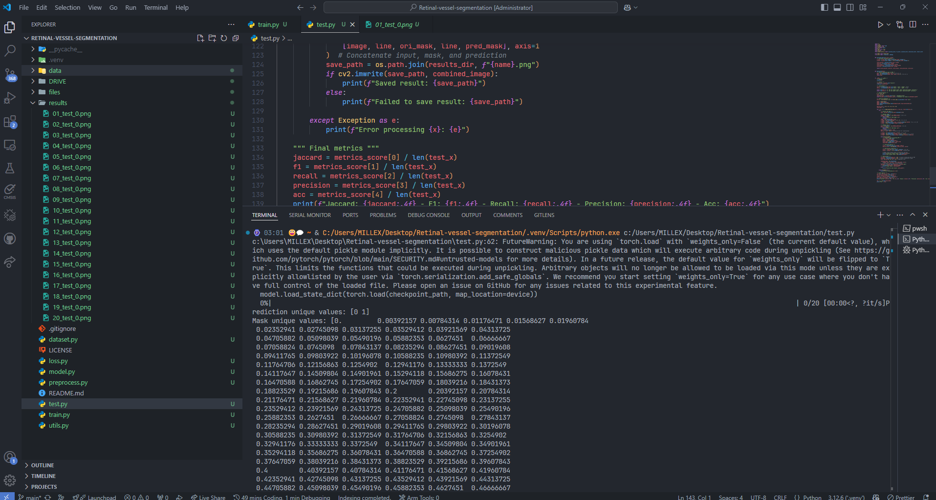
该代码用于 加载 U-Net 语义分割模型,进行推理并评估模型性能,主要功能如下:
- 计算评价指标 (
calculate_metrics)- 计算 Jaccard(IoU)、F1 分数、召回率、精准率、准确率,用于衡量分割质量。
- 先 Sigmoid 处理输出,将概率值转为二值掩码 (
>0.5)。
- 读取并处理测试数据
- 读取 测试集图像 (
test_x) 和掩码 (test_y),确保数据完整性。 - 进行 图像预处理:
- 归一化(
/255.0)。 - 调整形状(
(H, W, C) → (C, H, W))。 - 转换为
torch.Tensor送入模型。
- 归一化(
- 读取 测试集图像 (
- 加载 U-Net 进行推理
- 加载已训练模型 (
build_unet),从checkpoint.pth读取权重并转为 推理模式 (eval())。 - 遍历测试数据:
- 记录 推理时间(用于计算 FPS)。
- 计算 预测掩码(通过
torch.sigmoid()转换为二值)。 - 计算 分割评价指标 并累计。
- 加载已训练模型 (
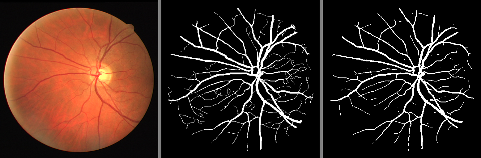
- 结果可视化与保存
- 生成 可视化图像,包含:
- 原始输入图像
- 真实掩码
- 预测掩码
- 采用
cv2.imwrite()将结果保存至results/目录。
- 生成 可视化图像,包含:
- 计算最终性能指标 - 计算 平均 Jaccard、F1、召回率、精准率、准确率,评估整体性能。 - 计算 平均 FPS,衡量模型推理速度。
结果展示
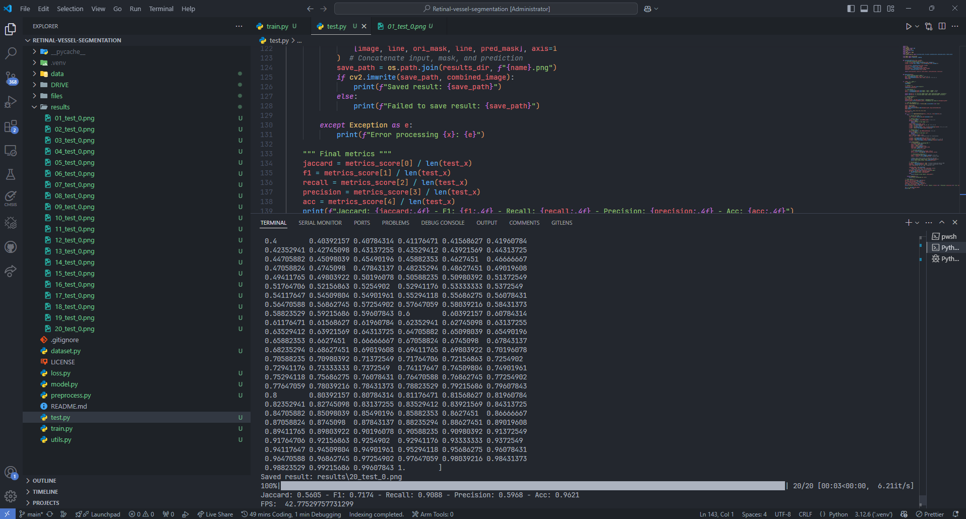
Jaccard: 0.5605
F1: 0.7174
Recall: 0.9088
Precision: 0.5968
Acc: 0.9621
FPS: 42.77529757731299
小结
U-Net 是比较早的使用多尺度特征进行语义分割的模型之一,其U形结构也启发了后面的很多算法。
与其他图像分割网络相比,U-Net模型的特点包含以下几点。
- 可以用于生物医学图像分割。
- 整个特征映射不是使用池化索引,而是从编码器传输到解码器,然后使用Concatenation串联来执行卷积。
- 模型更大,需要更大的内存空间。
总的来说,是一个很有意思的项目,欢迎讨论!